Introduction
Time series analysis involves examining datasets that are collected over time to identify meaningful patterns and variations. These variations can be broadly classified into long-term and short-term components. Recognizing and analyzing these components is crucial for effective forecasting, which enables data-driven decision-making across various domains.
1. Components of Variation in Time Series
Time series data exhibit different forms of variation, categorized as follows:
A. Long-Term Variations
- Trend (T):
A trend represents the long-term progression of a time series. It indicates whether the data exhibit an overall upward, downward, or stable movement over time. Trends can be linear or nonlinear and are fundamental in understanding the underlying direction of a dataset. - Cyclical Variation (C):
Cyclical variations are fluctuations that occur over periods longer than one year. These are generally associated with economic or business cycles and reflect alternating phases of expansion and contraction. Unlike seasonal variations, cyclical changes do not follow a fixed periodic schedule.
B. Short-Term Variations
- Seasonal Variation (S):
Seasonal variations are predictable and recurring fluctuations within a year. These patterns typically occur on a monthly, quarterly, or weekly basis. Common examples include increased retail sales during festive seasons or higher electricity consumption during summer. - Irregular Variation (I):
Irregular or random variations are unpredictable and do not follow any systematic pattern. These are caused by unforeseen events such as natural disasters, strikes, or policy changes, and represent the residual fluctuations in a time series.
2. Forecasting Techniques in Time Series Analysis
Forecasting methods aim to predict future values based on historical data patterns. The major forecasting techniques include:
A. Moving Averages
Moving averages are smoothing techniques used to reduce short-term fluctuations and highlight longer-term trends.
- Simple Moving Average (SMA):
Calculates the average of a fixed number of past observations. For instance, a 3-period SMA averages the current and two preceding values. - Weighted Moving Average (WMA):
Assigns varying weights to past observations, typically giving more importance to recent data points. - Exponential Moving Average (EMA):
Similar to WMA but assigns exponentially decreasing weights to older observations, responding more quickly to recent changes.
B. Regression Analysis
Regression analysis involves determining the relationship between a dependent variable and one or more independent variables. It is used to model trends and make forecasts based on known relationships.
C. ARIMA (Autoregressive Integrated Moving Average)
ARIMA is a sophisticated statistical model that combines autoregressive (AR), integrated (I), and moving average (MA) components. It is particularly effective for forecasting time-dependent data that may be non-stationary.
D. Machine Learning Models
Machine learning techniques, including neural networks (e.g., Recurrent Neural Networks and Long Short-Term Memory models), are increasingly used in time series forecasting. These models can capture complex, nonlinear patterns in data and often outperform traditional methods when sufficient historical data are available.
3. Applications of Time Series Analysis
Time series analysis is employed in a wide range of fields. Some notable applications include:
A. Finance
- Stock Market Analysis: Forecasting stock prices and identifying market trends.
- Economic Forecasting: Projecting GDP, inflation, and business cycles.
- Risk Management: Evaluating financial risks due to market volatility.
- Algorithmic Trading: Automating trading decisions using predictive models.
B. Economics
- Business Cycle Analysis: Detecting periods of economic expansion and contraction.
- Consumer Behavior Analysis: Forecasting demand based on historical purchase data.
- GDP Forecasting: Predicting economic growth using macroeconomic indicators.
C. Meteorology and Climate Science
- Weather Forecasting: Predicting weather conditions based on past data.
- Climate Modeling: Analyzing long-term climate trends and climate change.
- Environmental Monitoring: Tracking pollution levels and environmental impacts.
D. Healthcare
- Patient Data Analysis: Monitoring vital signs and disease progression.
- Disease Outbreak Prediction: Forecasting the spread of infectious diseases.
- Healthcare Resource Planning: Estimating future demand for medical resources.
E. Engineering and Manufacturing
- Process Control: Enhancing operational efficiency and product quality.
- Predictive Maintenance: Anticipating equipment failures.
- Performance Monitoring: Assessing machinery performance through sensor data.
F. Retail and Supply Chain
- Sales Forecasting: Predicting future sales to manage inventory effectively.
- Demand Planning: Ensuring adequate supply of products.
- Inventory Management: Optimizing stock levels to balance demand and cost.
G. Other Applications
- Social Science Research: Studying demographic and societal trends.
- Energy Forecasting: Predicting energy demand for efficient distribution.
- Traffic Analysis: Managing traffic flow through predictive modeling.
- Quality Control: Detecting production defects early.
- Agricultural Yield Forecasting: Projecting crop yields based on environmental data.
Conclusion
Time series analysis is a powerful tool for understanding the structure and behavior of data collected over time. By decomposing data into trend, seasonal, cyclical, and irregular components, and applying appropriate forecasting techniques, organizations can make informed, forward-looking decisions. Its diverse applications—from finance to healthcare and engineering—demonstrate its significance across industries and disciplines.